Demo code available at: https://github.com/unionai/unionai-examples/tree/main/v2/tutorials/multinode_rl_grpo_lora.
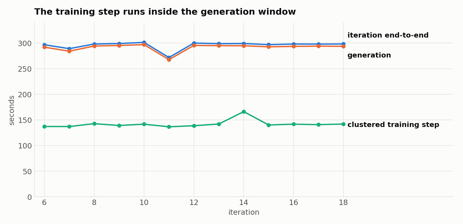
We built a complete GRPO loop on Flyte 2, complete with rollout generation, reward scoring, held-out evaluation, and a multi-node training step. It post-trained Qwen3-8B on GSM8K across two machines and eight GPUs. A quick gloss for anyone who doesn't live in this corner of ML: GRPO (Group Relative Policy Optimization) is the reinforcement-learning algorithm behind DeepSeek-R1, a rollout is one attempt the model makes at one problem, and GSM8K is a standard set of grade-school math word problems whose answers are numbers you can check automatically. What we wanted to find out was how much additional runtime that multi-node trainer actually costs you once the orchestrator is allowed to overlap it with generation, and in steady state the answer came out to almost nothing. Because the driver kicks off the next batch of rollouts before it awaits the training step, all 140 seconds of the eight-GPU update happen inside a generation window that was going to take 294 seconds anyway.
Our findings:
- Accuracy on held-out GSM8K questions, meaning ones the model never trained on, climbed from 60.9% to 85.9%, touching 92.2% at step 14.
- Since we were able to overlap rollout generation with multi-node training, a single step took 298 seconds, 294 of which was spent on rollout generation and 140 of which was spent on the multi-node training step.
- Running the same loop without overlapping the two costs 434 seconds per iteration instead.
- The training run spun up 1,323 individual cluster tasks, and none of them failed.
- Weight sync is a few megabytes of LoRA adapter written to object storage, so the trainer and the rollout fleet never talk to each other directly. LoRA (Low-Rank Adaptation) freezes the original model and trains a small set of extra weights alongside it, which is why the thing being shipped around each step is megabytes rather than the tens of gigabytes a full 8B model would weigh.
Steady-state iterations. The clustered training step is the bottom line, and the iteration tracks generation almost exactly, because the training runs inside it. Iterations 0 to 5 are left out; they carry the capacity wait described further down.
The rest of this post covers why the infrastructure is normally the hard part of RL, how we put the loop together, and the four things we got wrong before any of it worked.
The problem with multi-node RL today
RL post-training with verifiable rewards, usually shortened to RLVR, is where the frontier has moved, and the recipe itself isn't complicated: have the model attempt problems whose answers you can check, score the attempts, push the good ones up and the bad ones down, then repeat. The verifiable part means no human or judge model has to grade anything, because a math answer is either the right integer or it isn't. GRPO is the standard choice for the scoring half, and it amounts to a few dozen lines of math. Its trick is in the name, since it scores each attempt relative to the other attempts at the same prompt — six tries at one problem become six numbers saying which tries beat the group average, and those numbers are the advantages that show up throughout the code below.
The infrastructure is where it gets ugly. A real RL loop needs three things running at the same time:
- A rollout fleet — GPUs with the model resident, generating attempts. This is where most of your wall-clock goes; 70–80% is typical.
- A trainer — often several machines, either because the policy (the model being trained) has outgrown one GPU or because you want bigger batches per step.
- A controller — a long-lived process that decides what runs when, tracks in-flight work, ships new weights to the generators, and recovers when something dies.
Outside the big labs, that third piece is almost always a script, built out of Ray actors, thread pools and tmux windows. It tends to be the buggiest part of the stack, it rarely resumes cleanly, and when a GPU dies at 3am you lose the overnight run. We wanted to see how much of it disappears if you let the orchestrator do that job instead.
Only the trainer needs to be multi-node
The decision that makes everything downstream simple is that weight sync here isn't a network protocol at all.
We train a LoRA adapter rather than the full model, so the base weights stay frozen and what the trainer produces each step is a few megabytes of adapter. That's small enough to write to object storage and let the generators pick it up on their next request, which means there's no NCCL broadcast from trainer to rollout fleet, and the two never have to be scheduled together, wired together, or even aware of each other. NCCL is NVIDIA's library for shipping tensors straight between GPUs, and it's how full-weight trainers normally push fresh weights to their generators. It's fast, but it needs both sides alive and connected at the same moment, which is exactly the coupling we wanted to avoid.
So the fleet ends up looking like this:
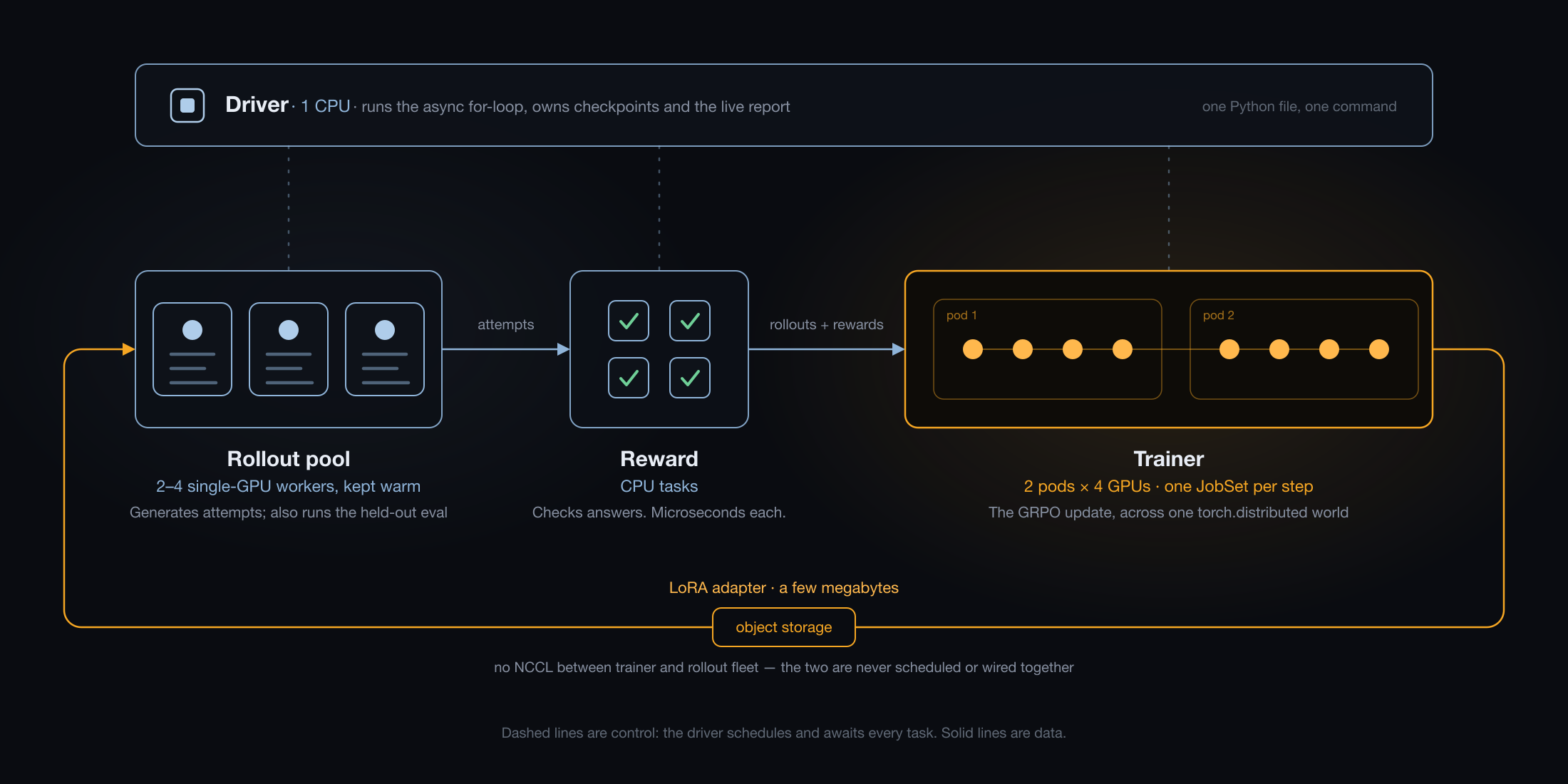
The driver sits on the control plane and never touches the data: it schedules each task and awaits the result. Attempts flow from the rollout pool through reward scoring into the training step, and the only thing coming back the other way is the adapter, which travels through object storage rather than over the network.
The trainer is the only row that needs more than one machine. In Flyte 2 each of these is a `TaskEnvironment`, which is just a hardware and software spec, and the multi-node one is a `ClusteredTaskEnvironment`:
Every call to a task in that environment emits a single Kubernetes JobSet, which is the Kubernetes primitive for a group of pods meant to start and stop as a unit. Inside it sit eight processes, bootstrapped by `torchrun` and rendezvoused into one `torch.distributed` world, started together and failed together. Each process drives one GPU and is called a rank, and eight of them together make a world size of eight, which is the vocabulary PyTorch uses for distributed training. You write one Python function and it runs on every rank, so moving from single-GPU to eight-GPU training is mostly a matter of that declaration — the body of the function barely changes.
The controller is just an async for-loop
The part that surprised us most was how little the controller turned out to be. It's the driver task, and it's an ordinary async Python function:
The middle line is where the whole async-RL trick lives. `asyncio.create_task` schedules generation of the next batch and returns immediately, so when the driver then hits `await train_step_clustered(...)` and parks there for minutes while the JobSet schedules, pulls its image, loads the model and trains, that parking hands control back to the event loop, which spends those minutes driving the generation task instead. Two things make progress at once on a single thread, and they can do that because the driver isn't computing anything itself — it's waiting on remote work, and waiting is free.
The `pipelined=False` switch we used to measure the benefit is the same statement moved eight lines down, after the training call. Same work and the same durations, except that now the two never coexist, so an iteration costs their sum rather than their maximum.
Because the driver is a task rather than a script, it also gets a few things a script wouldn't. Every generation and training call is traced as its own action in the run and grouped by iteration, with its own logs, inputs and outputs, and the loop checkpoints each iteration so a preempted driver picks up mid-run instead of starting over.
Overlapping forces you to fix the math
This is the part most "async RL" demos skip. When the driver launches generation of batch N+1, training on batch N hasn't finished, so the newest weights don't exist yet and the generators necessarily use the previous ones. By the time batch N+1 comes back and its turn to be trained on arrives, the policy has advanced by one update, so that batch was written by a slightly older model than the one it's about to update. This isn't a race condition to be tightened away; it happens every iteration by construction, and it's the price of the overlap that makes the loop fast in the first place.
It matters because policy-gradient methods are on-policy, which means the math behind them assumes your samples came from exactly the model you're updating. The simple policy-gradient loss everyone starts with
is only valid when the attempts came from exactly the policy being updated. Under pipelining they didn't, so the gradient you compute is quietly wrong. Nothing crashes and the loss stays a perfectly ordinary-looking number, which is what makes this easy to ship by accident. If you want to read around it, the terms to search are on-policy versus off-policy reinforcement learning.
The fix is the actual GRPO objective, and it needs one thing from the generator: what the model thought at the time it wrote each token. So `generate` records the sampling log-probabilities out of vLLM, the inference engine the rollout workers run on, into every rollout, and the trainer uses them. Those probabilities belong to weights that no longer exist by the time training happens, so unless the generator writes them down as it samples, there's no getting them back.
The ratio is importance sampling, a standard statistical move for estimating an average under one distribution using samples drawn from another, where you weight each sample by how much more or less likely it was under the distribution you actually care about. Here that means re-weighting each token by how far the current policy has drifted from the one that sampled it, which is what makes an estimate drawn from the wrong distribution unbiased again. The clip refuses to trust corrections beyond ±20%, so a token whose probability has moved a long way stops contributing rather than contributing a wildly scaled gradient, and it's the same clipping idea PPO introduced. The KL term measures how far the tuned model has wandered from the original and acts as a leash against drifting into whatever degenerate output happens to game the scorer, with `k3` being a low-variance way of estimating that distance. Because we compute it against the base model by simply disabling the adapter, there's no second model sitting in memory.
One detail deserves more attention than it usually gets, which is that a single token id can sink the whole thing. vLLM tokenizes the prompt and the completion separately, so if the trainer re-tokenizes the concatenated text, boundary tokens can merge and every position after them shifts. The importance ratio would then be comparing different tokens, and it would be garbage in a way that still runs perfectly happily. The rollouts therefore carry vLLM's exact token ids and the trainer feeds the model those, never re-tokenized text. Across all twenty steps the measured ratio came out at 1.000 ± 0.0003, which is what tells us the alignment is right; if it were off, the ratios would be wild.
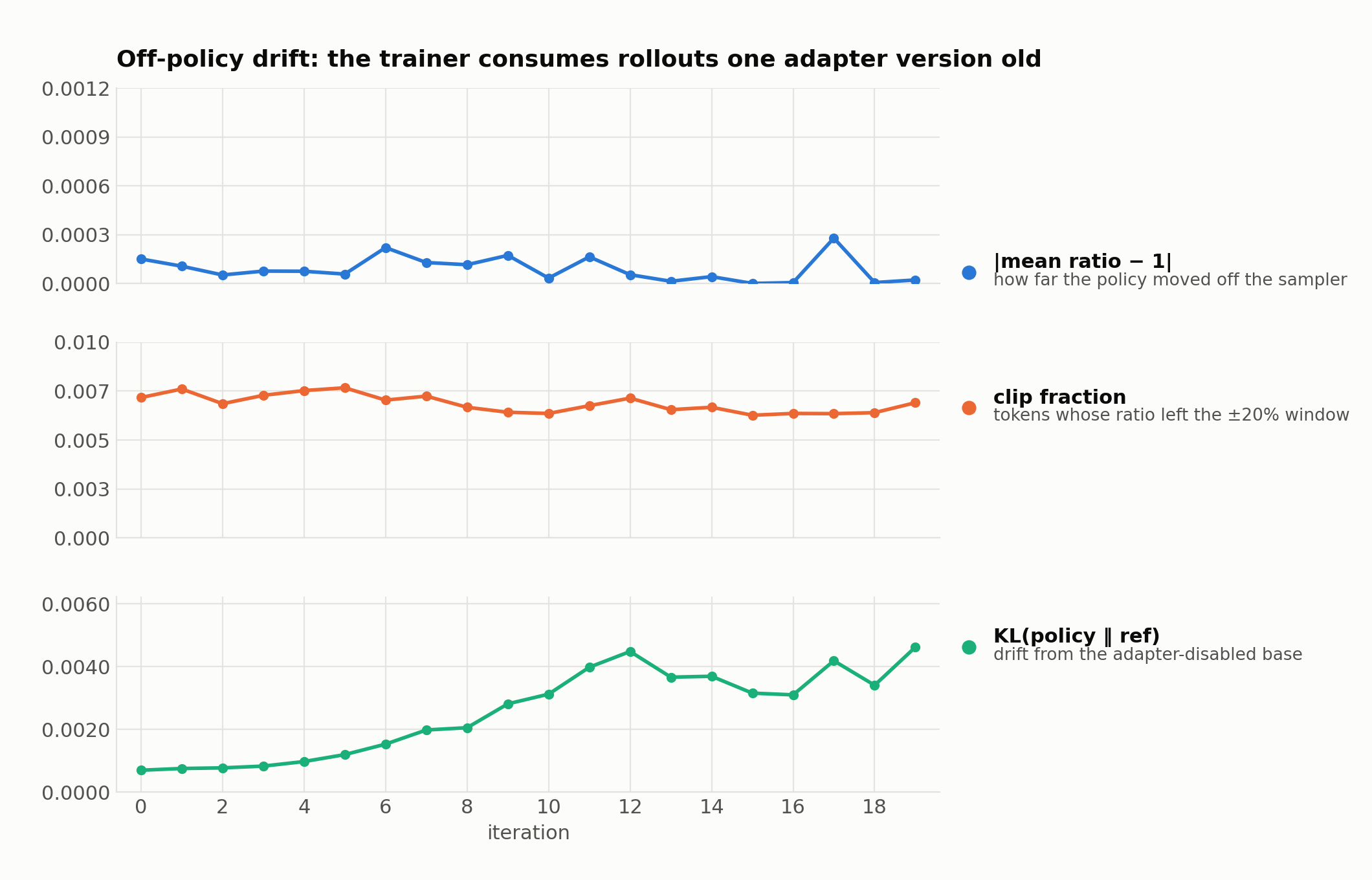
The three staleness signals across the run, each panel labelled on the right. The importance ratio never leaves 1.000, which is what says the token alignment is right. The clip engages on well under one percent of tokens. KL against the frozen base grows steadily and stays small.
The bug that a passing test hid
Our first smoke test passed end to end, and it shouldn't have reassured us.
PyTorch's DDP (Distributed Data Parallel, the usual way to run one model across many GPUs) synchronizes gradients inside every `backward()` call, so the eight ranks are constantly meeting up to average their gradients. Those meetings are called collectives, and every rank has to turn up to every one of them, which means all eight have to call `backward()` the same number of times or the ones that arrive wait forever for a rank that is never coming. The natural way to write a GRPO step runs straight into that:
Which attempts have zero advantage depends entirely on the data. Because the advantage is measured against the other attempts at the same prompt, a prompt where all six score identically produces six zeros and teaches the model nothing. Each rank gets a contiguous slice of the batch, so rank 0 doing three backwards while rank 1 does five is the expected case rather than an edge case, and at eight ranks with real reward variance it deadlocks immediately.
It didn't deadlock in our smoke test because the toy setup was small enough that every group scored identically. Every advantage was zero, every rank did zero backwards, and the gradient path was never exercised at all, so the test passed by not running the thing it was meant to be testing.
The fix is the documented `no_sync` pattern:
Backwards inside `no_sync()` carry no communication, and the first forward-backward after the context syncs everything, so every rank unconditionally runs one dummy 1-token forward and a zero-scaled backward, and the collective count comes out identical by construction, including on a rank whose shard is empty.
The shortcut you'll be tempted by — summing the losses, doing one backward, and adding `0 * sum(p.sum())` to cover empty shards — doesn't work, for two reasons. It retains every sample's autograd graph until the end, and that dummy term never passes through `DDP.forward`, so DDP's reducer isn't prepared for the iteration. You end up with the same class of bug one layer down.
The regression test now runs two processes on CPU using gloo, the CPU backend for the same collectives NCCL handles on GPUs, with an adversarially empty shard on rank 1, and asserts that the gradients come out identical and correctly normalized. It takes seconds and needs no GPU.
What the numbers said
The stress run was twenty steps of 32 prompts × 6 attempts, 512-token completions, GSM8K, with an 8B policy spread over two machines holding four NVIDIA L40S GPUs each.
Held-out accuracy started at 60.9%, peaked at 92.2% on step 14 and settled at 85.9%, measured on sixty-four questions the model never trained on, using greedy decoding, where the model always takes its single highest-probability next token so the score doesn't wobble between runs.
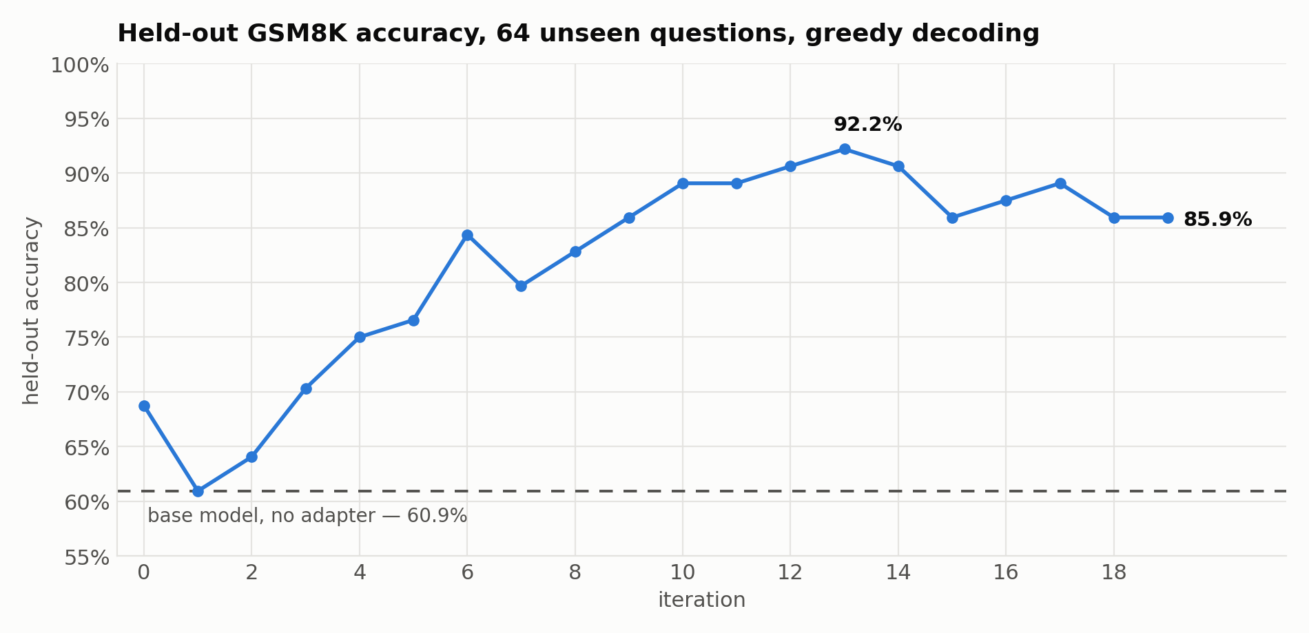
Every point is a fresh greedy pass over the same sixty-four held-out questions. The dashed line is the base model with the adapter disabled.
On timing, a steady-state iteration came to 298 seconds against 294 for generation and 140 for the clustered training step. The next batch's generation starts a second or two before the training step and finishes about two minutes after it, so the JobSet's entire lifetime fits inside. Run sequentially, the same iteration takes 434 seconds.
The health signals all behaved. The importance ratio held at 1.000 ± 0.0003, the clip fired on 0.6–0.8% of tokens, KL climbed smoothly from 7e-4 to 4.6e-3, and gradient norms sat around 0.02. The number of attempts carrying a learning signal fell from 180 to roughly 100 out of 192 over the run, as more prompt groups became all-correct. Once every attempt at a prompt succeeds there's nothing left to rank them by, so the advantage collapses to zero and that prompt stops teaching the model anything, which is textbook GRPO saturation and the signal that it's time to move to harder prompts.
Four things we got wrong
1. At small scale, pipelining does nothing, and that isn't a flaw in the idea.
Our first pipelined run used a 0.6B model, where generation took around 60 seconds and the training JobSet took anywhere from 200 to 640. The overlap worked exactly as designed and saved us about a minute out of ten. The claim only holds when generation is the long pole, which is the regime real RL runs in and not the regime a toy demo runs in, so scaling the rollout batch until generation dominates isn't just making the demo bigger — it's the configuration in which the claim becomes true at all.
2. A multi-node step waits for the entire cluster it asked for.
Our first training step spent three and a half hours waiting to start, almost none of it compute. Karpenter, the autoscaler that provisions fresh nodes for a Kubernetes cluster on demand, couldn't get two `g6e.12xlarge` instances out of the cloud provider for that long, and an eight-rank step can't begin until all eight ranks exist, so the step's start time is set by the last node to arrive.
What happened around that is the part worth reporting. The driver parked on the await and spent those hours driving generation instead, the next batch's rollouts finished on schedule, no task failed, and training began the moment capacity arrived. Capacity for a specific instance type in a specific region is the scarcest thing in this entire setup, so check it before a long run, set up a nodepool that will accept several 4-GPU instance types, and warn the tenant owner before you pin two 4-GPU nodes for an afternoon.
3. Our accuracy gain measures the floor we chose, not the ceiling we reached.
61% is low for an 8B model on GSM8K — published numbers are north of 90% once you use a chat template, the conversational formatting a model was tuned to expect, and give it room to reason before answering — and that was deliberate. A model already sitting at 92% has nowhere to go and the accuracy curve would be flat noise, so we used a plain prompt with no chat template and a strict `#### <integer>` answer format, which left visible headroom for RL to close.
Read the curve as evidence that the loop learns rather than as a claim about the model's mathematical ability. The gain is real and it's on questions the model never saw, but in absolute terms it's a return to roughly where a well-prompted 8B already sits.
4. The staleness we designed around turned out to be invisible.
Clip fraction was identical whether we ran pipelined or sequential, because at this learning rate one step of staleness moves the policy so little that the importance correction is nearly a no-op. The ~0.6% of tokens that do fall outside the clip window aren't staleness at all — they're vLLM and PyTorch computing the same probabilities and disagreeing slightly, which is the training/inference mismatch people write papers about, and the chart measures it for free.
The correction still earns its place, though. It's what keeps the design safe at a higher learning rate, with more epochs per step, or with a deeper pipeline, and it's what makes the pipelining a real optimization rather than a silent approximation.
Try it
The tutorial ships with two profiles behind a single environment variable.
Start with `smoke`. It exercises the clustered JobSet, the real objective, the eval and the report in about twenty-five minutes, so if something's wrong with your cluster you'll find out cheaply. There's also a Colab notebook that drives the whole thing as a pure client, with no torch and no CUDA locally — just an API key and a link to a live report carrying the accuracy curve, the drift chart and the timing breakdown.
Where this goes next
A few directions, roughly in order of how much you'd learn from them.
Harder prompts matter most, because once half your batch stops carrying a learning signal the curriculum is the bottleneck rather than the compute. Bigger policies come next: an 8B model fits on a single 48GB card in bf16, a 16-bit number format that halves memory use against full precision, so plain DDP suffices. Past roughly 30B you'll want FSDP (Fully Sharded Data Parallel), which splits the model itself across GPUs instead of replicating it, and on a TCP interconnect you'll want hybrid sharding, where you shard within a machine and replicate across machines so cross-node traffic stays at adapter scale. Full-weight RL is the harder jump, since once LoRA capacity runs out you need multi-GB weight handoff and vLLM's sleep/wake cycle, and that's the point where trainer and rollout fleet finally do have to live in one gang. Executable rewards are the cheapest thing to try — ours checks an integer, but you could swap it for running generated code against unit tests, or SQL against a database, and because the reward is just a task it scales, retries and versions like one.