GPUs in MLOps: Optimization, Pitfalls, and Management

Graphics Processing Units have roots deep in gaming, but they’re serious business when it comes to machine learning. First designed to accelerate compute-intensive graphical calculations, these specialized circuits can handle all sorts of data crunching — and their remarkable capacity for parallel processing makes GPUs essential tools for the biggest data tasks.

That includes the demands of machine learning, where GPUs can distribute the work of training data. ML just wouldn’t be possible without that horsepower! 

Using GPUs well for ML requires some techniques and debugging strategies, it’s not free from pitfalls. In this post, we’ll look at coding for GPUs and note some common pitfalls along with their solutions when using GPUs at scale.

Because NVIDIA currently dominates the ML/DL ecosystem, we’ll focus here on NVIDIA devices — ROCm and OpenCL are super-capable GPU stacks and deserve their own blog post.

To start, let’s explore the GPU! What makes it different from a CPU anyway?

In the graphic above, you can see a conventional 4-core CPU. You may notice that the GPU has a few more than four! The GPU cores in an Nvidia device are called CUDA cores. While a CPU adeptly handles multiple tasks, a GPU excels at executing thousands of simpler tasks concurrently. It’s like comparing a small team of generalists to an army of specialists.

We won’t be diving into the extreme details of what a GPU is; there are other fantastic blog posts;. However it’s worth looking at an example of CUDA code and what makes it so different.

Let’s code: The classic way vs. the CUDA way

Let’s do something … interesting. We’ve got a list of 1 million integers (randomly initialized), and we want to perform a series of math operations on each of them. Let’s look at the standard Python way of approaching the problem as well as the JAX equivalent.

Classical Python approach

import time
import random
import math

# Generate a list of 1 million random integers between 1 and 100
inputs = [random.randint(1, 100) for _ in range(1000000)]

# Define a list of 500 math operations
operations = [math.sin, math.cos, math.tan, ...]  # This should contain 500 math functions

start_time = time.time()
outputs = []
for item in inputs:
    result = item
    for operation in operations:
        result = operation(result)
    outputs.append(result)

end_time = time.time()

print("Output sample:", outputs[:5])
print("Estimated Compute Duration (Classic):", end_time - start_time, "seconds")

# Completed in 7.8 secs

‍

JAX-based approach

import jax
import jax.numpy as jnp
import numpy as np
import time
import random

# Ensure computations are on the GPU
jax.devices('gpu')

# Generate a list of 1 million random integers between 1 and 100
inputs = np.array([random.randint(1, 100) for _ in range(1000000)], dtype=np.float32)

# Define a list of 500 math operations
operations = [jnp.sin, jnp.cos] * 250  # This is just a placeholder; you can replace with actual operations

@jax.jit
def apply_operations(input_array):
    def apply_ops_to_item(item):
        result = item
        for operation in operations:
            result = operation(result)
        return result
    return jnp.vectorize(apply_ops_to_item)(input_array)

start_time = time.time()
outputs = apply_operations(inputs)
end_time = time.time()

print("Output sample:", outputs[:5])
print("Estimated Compute Duration (JAX):", end_time - start_time, "seconds")

#Completed in 0.15 secs

JAX is pretty cool right? It’s a nice way to quickly describe complex, efficient computations as simple python - and seamlessly converts into CUDA code when passed to a GPU.

In this example, each row can be computed independently of any other row, which makes this problem parallelizable — perfectly suited for computation on a GPU.

But why should we use GPUs for ML?

At the core of machine learning — especially deep learning — lie matrices. Large, complex matrices. Whether we’re forwarding inputs through neural network layers or back-propagating errors, we’re engrossed in matrix operations.

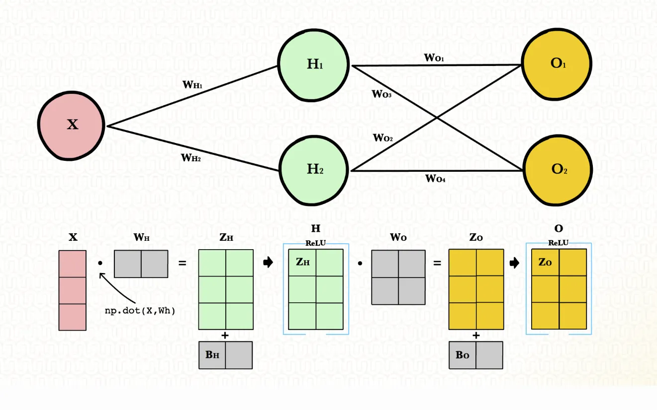
Like the previous example, matrix multiplication row wise is parallelizable. Instead of having to execute every row sequentially, we can calculate them all at the same time.

NVIDIA’s CUDA and cuDNN are the secret sauces that make GPUs even more potent for ML tasks.

For a change, lets have a glimpse into matrix multiplication using CUDA, written in C:

__global__ void matrixMul(float *A, float *B, float *C, int N) {
    int row = blockIdx.y * blockDim.y + threadIdx.y;
    int col = blockIdx.x * blockDim.x + threadIdx.x;
    float sum = 0;
    for (int i = 0; i < N; i++) {
        sum += A[row * N + i] * B[i * N + col];
    }
    C[row * N + col] = sum;
}

// Usage
dim3 threadsPerBlock(16, 16);
dim3 blocksPerGrid(N / threadsPerBlock.x, N / threadsPerBlock.y);
matrixMul<<<blocksPerGrid, threadsPerBlock>>>(d_A, d_B, d_C, N);

Especially when paired with optimizations from cuDNN, this setup makes deep learning computations blazingly fast.

Here be dragons, however

GPU-accelerated workflows may be fast, but you may run into trouble using them outside local use on your own computer. One example of this is “surprise OOM errors,” out-of-memory errors caused by heterogenous use without careful planning.

Hypothetical Machine Specs:

• GPU Memory: 12 GB

Scenario:

User A and User B are both running deep learning models on this machine.

User A’s Model:

• A large neural network for image classification
• Requires 9 GB of GPU memory for its operations

User B’s Model:

• A smaller neural network for text classification
• Requires 5 GB of GPU memory for its operations

Situation 1: Parallel execution (OOM error)

User A’s configuration:

import torch

# Define and load User A's large model
model_A = torch.nn.Sequential(
    # ... many layers here ...
)
model_A.cuda()  # Moves the model to the GPU

‍

User B’s configuration:

import torch

# Define and load User B's smaller model
model_B = torch.nn.Sequential(
    # ... some layers here ...
)
model_B.cuda()  # Moves the model to the GPU

In this situation, both User A and User B attempt to load their models onto the GPU simultaneously. The combined memory requirement is 9GB + 5GB = 14GB, which exceeds the GPU’s capacity of 12 GB. This will trigger an OOM error.

Situation 2: Sequential execution (no OOM error)

Now, let’s assume both users decide to run their models one after the other, instead of simultaneously.

User A’s configuration:

import torch

# Define and load User A's large model
model_A = torch.nn.Sequential(
    # ... many layers here ...
)
model_A.cuda()  # Moves the model to the GPU

# Run training or inference
# ...

# After completion, free up GPU memory
del model_A
torch.cuda.empty_cache()  # Clears up the cached memory

‍

After User A’s operations complete and the memory is cleared, User B starts their operations.

‍User B’s configuration:

import torch

# Define and load User B's smaller model
model_B = torch.nn.Sequential(
    # ... some layers here ...
)
model_B.cuda()  # Moves the model to the GPU

# Run training or inference
# ...

In this sequential setup, at no point does the GPU memory usage exceed its 12 GB capacity. Hence, there’s no OOM error.

This example illustrates how runtime configurations and the order of operations can influence memory consumption on a GPU. Running tasks sequentially and ensuring proper memory cleanup can prevent OOM errors in scenarios where parallel execution might fail.

Effective strategies for GPU resource allocation and management

In the heady rush to adopt GPUs for ML tasks, users may overlook the challenge of managing these powerful resources effectively. Despite their sheer computational advantage, GPUs’ potential can be squandered without proper resource allocation and management. Let’s dive into the strategies that can help you maximize the benefits of your GPU resources.

If your model is small

Assuming you're not training a LLM from scratch, you might be able to fit multiple instances of your model on a single GPU, it might even be able to run locally. If that’s the case, it might be helpful to do the following:

• Profile before deploying: Use profiling tools like NVIDIA’s ‘nvprof’ to get insights into the memory and compute utilization of your models. This helps in understanding bottlenecks and can guide resource allocation decisions. You can even profile your Python code (pytorch or tensorflow work!) with ‘nvprof python3 your_script.py’
• Validate memory footprint: Before deploying to a shared or constrained environment, check the memory footprint of your model with tools like torch.cuda.memory_allocated() for PyTorch or tf.profiler.experimental.Profiler for TensorFlow. Small models can sometimes have hidden memory costs, especially when tied to larger frameworks or with auxiliary data structures. Understanding the total GPU memory requirement ensures you allocate resources appropriately and avoid surprise OOM errors even with smaller models.
• Model optimization and pruning: Before deploying, consider techniques like model pruning or quantization. Tools such as TensorFlow’s Model Optimization Toolkit or PyTorch’s pruning utilities can help reduce the size of your model without significantly compromising accuracy.

As an example, here’s how that can be done in PyTorch:

import torch
import torch.nn as nn
import torch.nn.utils.prune as prune

# Define a simple model
class SimpleNet(nn.Module):
    def __init__(self):
        super(SimpleNet, self).__init__()
        self.conv1 = nn.Conv2d(3, 64, kernel_size=3, stride=1, padding=1)
        self.fc1 = nn.Linear(64*32*32, 10)

    def forward(self, x):
        x = self.conv1(x)
        x = x.view(x.size(0), -1)
        x = self.fc1(x)
        return x

# Create a model instance
model = SimpleNet()

# Use global unstructured pruning on the 'weight' of conv1 layer
# Prune 30% of the connections based on their absolute magnitude
prune.global_unstructured(
    [model.conv1], 
    pruning_method=prune.L1Unstructured, 
    amount=0.3,
)

# You can inspect the pruned model's weights
print(model.conv1.weight)

# To make the pruning permanent, remove the 'weight_orig' and 'weight_mask' attributes
prune.remove(model.conv1, 'weight')

This not only reduces memory consumption but can also lead to faster inference times. Remember, a leaner model often translates to a more efficient deployment, especially in environments where resources are at a premium.

If your model is not so small

Dealing with larger models presents a different set of challenges. They often come with significant computational demands, both in terms of processing and memory requirements. When your model starts to grow, these considerations can help ensure efficient GPU utilization and smooth operation:

• Distributed Training: When a model becomes too large to fit on a single GPU, or when training times become prohibitively long, it’s time to consider distributed training. Libraries like NVIDIA’s NCCL or frameworks like Horovod allow you to distribute your model and data across multiple GPUs or even multiple nodes. This parallelism can significantly accelerate training times.‍
• Gradient Accumulation: If your model’s mini-batch doesn’t fit into GPU memory, gradient accumulation can be a lifesaver. Instead of reducing the mini-batch size (which can affect model convergence), process smaller chunks of your mini-batch and accumulate gradients over iterations before performing a weight update.

optimizer.zero_grad()  # Reset gradients tensors
for i, (inputs, labels) in enumerate(dataloader):
    outputs = model(inputs)
    loss = criterion(outputs, labels)
    loss.backward()  # Backpropagate the gradients
    if (i+1) % accumulation_steps == 0:  # Wait for several backward steps
        optimizer.step()  # Now we can do an optimizer step
        optimizer.zero_grad()  # Reset gradients tensors

• Mixed-precision training: Training in mixed precision, using both 16- and 32-bit floating point types, can improve model training speed and reduce memory usage, speeding training without costing significant model accuracy. NVIDIA’s Apex library offers utilities to enable mixed-precision training with a few lines of code.
  
• Use gradient checkpointing: For models with deep architectures, gradient checkpointing can be invaluable. This technique trades compute for memory, allowing you to fit much larger models onto GPUs by re-computing intermediate activations during the backward pass.
  
• On-the-fly data loading: Rather than pre-loading your entire dataset into GPU memory, use data generators or PyTorch’s ‘DataLoader’ with the ‘pin_memory’ option set to ‘True’. This ensures that data is loaded on the fly and moved to GPU memory in batches, reducing overall memory consumption.
  
• Model Parallelism: For models that are too large to fit on a single GPU, consider model parallelism. This involves splitting your model into distinct parts and placing each part on a different GPU. Frameworks like PyTorch and TensorFlow offer native support for model parallelism.
  

Remember, as models grow in complexity and size, the nuances of GPU resource management become even more critical. Efficiently leveraging accelerators can make the difference between a model that’s viable in production and one that remains confined to the drawing board. Always keep a close eye on GPU metrics, iterate, and optimize.

Build your own GPU-accelerated K8s

Harnessing the power of GPUs in a Kubernetes ecosystem requires not just the right tools but also a deep understanding of the intricacies involved. If you’re keen on building GPU support yourself, Kubernetes offers an array of specialized tools that can be customized to fit unique requirements. Below are some foundational tools and services that you can use and potentially extend.

Rolling out your NVIDIA GPU support: While NVIDIA already provides a GPU operator for Kubernetes, understanding its underpinnings can be valuable. This operator essentially streamlines the GPU provisioning process, manages runtimes, and oversees device plugin discovery and monitoring. If you wish to modify or build upon this, understanding how GPU resources are managed akin to CPU and memory is crucial.

The GPU Operator also bundles in the DCGM Exporter; and MIG deployer and a number of other metric gathering systems.

# To deploy the NVIDIA GPU Operator manually
helm repo add nvidia https://nvidia.github.io/gpu-operator
helm repo update
helm install --wait --generate-name nvidia/gpu-operator

Customizing Multi-Instance GPU (MIG) configurations: NVIDIA’s MIG allows for the division of a single A100 GPU into multiple GPU instances. While Kubernetes offers out-of-the-box support for MIG, diving deeper into configurations can allow for more tailored GPU instance allocations, especially useful for specific workloads.

apiVersion: v1
kind: Pod
metadata:
  name: custom-gpu-mig-pod
spec:
  containers:
  - name: cuda-container
    image: nvidia/cuda:11.0-base
    resources:
      limits:
        nvidia.com/gpu-mig-1g.5gb: 1

Or maybe you don’t have to! MLOps Orchestration

Setting up and maintaining a Kubernetes stack tailored for GPU orchestration is certainly a daunting endeavor. But what if you could focus on your core ML tasks, leaving the orchestration complexities to dedicated platforms? Enter ML orchestration platforms.

Kubeflow

• Pros: A comprehensive machine learning platform built on Kubernetes, Kubeflow provides tools for training, serving, and monitoring ML models, integrating seamlessly with popular ML libraries
• Cons: Its rich feature set brings complexity, making it potentially overwhelming for smaller projects

MLFlow

• Pros: MLFlow streamlines end-to-end machine learning workflows with its modular structure, supporting diverse ML libraries and offering tools for experiment tracking and model deployment
• Cons: While it’s versatile, it doesn’t offer the deep Kubernetes-native integrations that platforms like Kubeflow provide

Airflow

• Pros: A robust platform for orchestrating computational workflows and data-processing pipelines. With an extensive plugin system, it offers integrations with a multitude of systems
• Cons: Primarily designed with data engineering in mind. Integrating machine learning workflows might require additional legwork

TensorFlow Serving

• Pros: A dedicated tool from TensorFlow, TensorFlow Serving is optimized for serving machine learning models in production environments, requiring minimal setup
• Cons: It’s tailored exclusively for TensorFlow models, which can be limiting if your ecosystem involves multiple frameworks

Flyte

Emerging as a Kubernetes-native workflow automation platform, Flyte stands out with its ability to interoperate with systems like Airflow, Spark and Kubeflow. It leverages dedicated operators to spin up and tear down ephemeral clusters on demand, ensuring resource efficiency.

• Pros: Beyond its scalability and native Python SDKs, Flyte’s strength lies in its extensibility. It can capitalize on the best of Airflow, Spark, and Kubeflow, offering a versatile orchestration solution. The platform also emphasizes type-safety, ensuring data integrity
• Cons: As a newer entrant, it might not have all the features of established platforms, but its rapid evolution is bridging any gaps

Here’s a snapshot of how you’d define a GPU-enabled task and workflow in Flyte:

from flytekit import task, workflow
from flytekit.types.file import FlyteFile

# Defining a Flyte task that uses GPU
@task(
    requests=Resources(cpu="2", mem="500Mi", gpu="1"),
    limits=Resources(cpu="2", mem="500Mi", gpu="1")
)
def gpu_powered_task(input_data: FlyteFile) -> str:
    # Your GPU processing logic here
    pass

# Defining a Flyte workflow
@workflow
def gpu_workflow(data: FlyteFile) -> str:
    return gpu_powered_task(input_data=data)

Flyte’s intuitive structure and native Python SDKs simplify workflow management. Its inherent compatibility with Kubernetes ensures that GPU resource requests and limits are always honored.

In summary, while constructing your orchestration stack offers unparalleled flexibility, MLOps orchestration platforms can significantly reduce overhead. Your selection will hinge on your team’s know-how, your workflow’s complexity and your operational scale. Ensure your choice is aligned with both present requirements and future growth.